
Modelling pollutant density associated with surface water run-off
Industry representatives: Brooke Swaffer and Jacqueline Frizenschaf, SA Water Corporation
Moderators: Melanie Roberts, IBM Research – Australia, Melbourne; Tony Miller, Flinders University, Adelaide
Background
SA Water Corporation (SA Water) is a SA State Government owned water utility that manages the water collection, treatment and distribution network throughout South Australia. As part of this role they are responsible for ensuring that appropriate water quality standards are maintained for the water they supply to their customers. A significant source of SA Water’s raw water supply is surface water collected from a number of catchments throughout the state, but particularly catchments located in the Adelaide Hills. These catchments are almost exclusively privately owned land, and as a result, the associated land use arrangements are complex. They deliver source water that is highly variable in quality and can be difficult to treat. Agricultural enterprises dominated by livestock, in particular, can lead to the increased occurrence of undesirable microbial populations in the soil. Rainfall events can liberate these microbes from the soil and they may enter into streams from surface water run-off, and ultimately find their way into storage reservoirs. One of the tasks of water treatment is to remove or neutralise microbes that are potentially injurious to human health. Although it is always possible to treat raw water to a degree that neutralises these microbes, to do so can be costly. It is therefore desirable not to over-treat water beyond that which is necessary to neutralise the concentration of microbes actually present, with a suitable safety margin included.
Unfortunately, the determination of microbial population counts in raw water is a complex laboratory process, which is both costly and time consuming. Turn around times for assays are typically of the order of 2 – 3 days. Therefore such assays cannot be used for effective real-time control of water treatment. The problem that SA Water brought to the 2016 MISG centered around the ability to predict, in real time, the microbial concentrations in surface water runoff. Although microbial populations cannot be determined in real time, a number of other, more physical properties of surface water run off can be measured in real-time with reasonable reliability. These include (volumetric) flow rate, turbidity and electrical conductivity of the surface water, typically at some points in the major streams or creeks within a catchment. Precipitation (rainfall) can also be measured automatically at various points in the catchment. SA Water has progressively rolled out these kinds of real-time sensors at key locations within their catchments in recent years, and is now considering how they may be used to predict microbial concentrations.
The first step in order to do this is to collect microbial population count data that can be used to calibrate a prediction model. Historically this was done by a person physically collecting a 10L sample of raw water at key locations in a catchment. This was done both on a scheduled basis, that is at regular time intervals, and in response to rain events. This latter type of collection presented many practical difficulties, as rain events often occur at inconvenient times for staff availability. As a result, such samples were often collected sometime after the peak flow associated with the rainfall event had passed. Recently, SA Water have introduced automatic sample collecting at a small number of locations, which may obviate some of the logistical constraints of manual sampling procedures. (This equipment allows up to 24 samples of 10L each to be automatically collected at a single site.)
SA Water was able to supply data consisting of microbe counts and some of the above physical variables for a number of catchments. For some catchments this data went back ten years or so; however, the older data mostly only contained microbe count and flow rate. Only the more recent data also had data for the other physical variables mentioned above. The team was also cautioned that some of the older data might also be of suspect quality in some locations. On the whole, it was thought that the physical data that was measured by the automatic sensors would be the most reliable.
After an initial review of the problem that SA Water had presented, the MISG team formed into a number of sub-teams that each addressed a different aspect of this overall problem. It was noted that there is a significant body of literature on catchment models that seek to relate surface water run-off to rainfall, catchment topography, catchment hydrogeology and measures of catchment dryness. However, it was felt these were unlikely to be particularly relevant to this particular problem, as in this case measured hydrograph data is actually available.
Sub-team activities
The discussions of the various sub-teams will now be briefly summarised in the following subsections.
Statistical reliability of microbe counts
In discussions with SA Water the team soon realised that there were significant statistical questions relating to the microbe assay process. Although a standard laboratory procedure is being followed, it is common place for microbes to be “lost” in the assay process. In an attempt to quantify this, a known number of “marked” control microbes is added to the sample before assay. The number of these marked microbes that appear in the final count after laboratory processing is then used to gross up the corresponding count of unmarked microbes to arrive at a value that is then taken to be the “actual” microbe count in the original sample. This is based on the assumption that equal proportions of marked and unmarked microbes will be “lost”. Yields for the marked microbes of 30 – 50% are common, but yields both higher and lower also occur; thus, actual counts can be routinely scaled up by factors of 2–3.
In addition to these errors in the assay process itself, it is also to be expected that there is environmental variability. For example, it is SA Water’s belief that the microbes in the run-off may tend to clump together, so that it is unlikely that they will be uniformly distributed through the run-off stream. It is also likely that the microbe concentration may differ in different parts of the stream due to different flow hydrodynamic conditions (for example top and bottom differences, and mid-stream and edge differences). Bearing in mind that only a 10L sample is being collected from streams with flow rates of tens of cubic metres per second, or more, there are obvious questions about how representative any single sample may be. In an attempt to quantify this sampling error, some 40 sets of four “repeat” measurements were identified amongst SA Water’s data.
Using these repeat measures and some statistical models of both the sample collection and the microbe assay processes, some simulations were performed that yielded estimated confidence intervals on the microbe counts. These models predicted relative errors in the microbe count of around 30% in cases where there was a low yield of marked microbes. More specifically, Table 1 shows the relative error at one standard deviation based upon a Monte-Carlo simulation. However, a comparison with an analysis of the repeat measurements indicated that for slightly more than one-third of the 40 sets of four repeats, the variability between the four samples within the set was greater than the 99% percentile predicted by the theoretical simulations based on the assumed statistical models. This indicates that the data appears more variable than the statistical models looked at during the MISG would suggest, and that further work is required to better understand and quantify the sources of variability in the microbe count data.
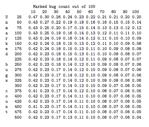
Table 1: Relative error in the final grossed-up microbe count at one standard deviation, based on a Monte Carlo simulation. The rows correspond to the original count of unmarked microbes, and the columns are the recovery rate of the 100 marked bugs.
Identifying microbe count correlates
Through a review of the physical processes involved and of the data available to the team, a number of potential correlates to the microbe count were assessed. These included flow rate (discharge), water level, turbidity, salinity and rainfall. It was also conjectured that there may be seasonal effects and also some dependence on the history of rain events in the previous few weeks or month. These latter two effects reflect the possible role of soil dryness, the saturation level of the soil and the ability of the microbe population in the soil to recover after previous rain events.
Two data analysis approaches were used to further explore these possible correlations. A Principal Compo- nent Analysis (PCA) led to the following observations:
- turbidity and discharge rate are the best variables to explain microbe concentration following rain events
- salinity (electrical conductivity) and soil dryness are the best variables to explain microbe concentration during non-rain periods, principally summer.
A linear correlation analysis suggested
- there is a general correlation of microbe count with flow rate (discharge)
- there appears to be a seasonal trend, with microbe count diminishing over the course of the year (autumn – spring), other factors being equal. This effect however is not standout, and needs to be treated with some caution.
- correlations were better for high flow rates and late season; and poorer for low flow rates.
Can flow rate and turbidity predict microbe counts?
The problem as presented to the MISG was expressed in terms of microbe concentration. This also is what is directly measured. However, a quantity that is probably of more direct practical importance is the microbial load, which is defined as the product of the microbe concentration and the flow rate. This describes the number of microbes that pass the sampling location per unit of time, and is a more direct measure of how many microbes are entering the water storage system.
One approach that was taken was to examine various plots of pollutant load against flow rate and turbidity for different catchments and different seasons or groups of seasons. Although this was not done exhaustively, a few observations were made for the cases that were examined.
- Microbial load is reasonably well predicted by flow rate on the basis of a visual examination of the plots.
- The general pattern of the plots is a flat region for low flow rates , and then a rising curve at higher rates. The specifics, for example, the extent of the initial flat region, depends on the catchment and also possibly on the season (year).
- There is not much effect of turbidity; in fact, the maximum microbial loads tend to occur at mid-range values of turbidity.
It was noted that these observations seemed most apparent for most recent datasets, say post-2012. In addition it was noted that the microbial count data was mostly collected on the rising edge of the hydrograph, seldom at peak flow rates. Thus, the plotted data probably did not cover the full range of microbial loadings, and so little could be said about what was happening at the highest flow rates.
Physical washout model of microbe concentration
There was some discussion of whether there was in effect an infinite supply of the microbe readily available in the soil for uptake by the run-off, or whether the microbe population could wash out over a season or during an extended rainfall event. Two simple models were developed to try to better understand what may be happening in this regard. Both models combined a trickle run-off model on a sloping terrain, a microbe take-up model for the run-off and a simple single stream flow model for the outflow of the catchment. Calculations were conducted to determine the shape of the count versus time curve compared to the run-off verses time curve using different initial microbe levels in the catchment during a single rainfall event and different assumptions concerning microbe take-up by the run-off. These calculations should enable comparison with data from a single event and also with seasonal data. There was insufficient time to pursue this further in the MISG. Further work has been done on this approach, which will be described in the final technical report.
Time delay between rainfall record and hydrography
As outlined above the team shied away from seeking to predict the hydrograph from the rainfall data; however, it was still thought useful to look at and compare the rainfall data and the subsequent hydrograph. This proved a useful exercise. Looking at a number of rainfall events over a variety of catchments showed that the pattern of peaks and troughs of the rainfall record and the subsequent hydrograph were quite similar. For example, the occurrence of multiple peaks in the hydrograph could be identified from the earlier rainfall record. The hydrograph lags the rainfall record by a delay that varies by catchment and season, ranging from 2 – 10 hours for the examples considered. Delays in summer tend to be longer, presumably due to soil dryness; whilst a second rainfall event close to an earlier one leads to a quicker response, presumably as the soil is already close to saturation.
Although no serious attempt was made to analyse the magnitude of rainfall and subsequent flows, the findings described above regarding hydrograph shape and lag raise the potential that the rainfall record can be a practical tool for predicting the onset and pattern of the subsequent hydrograph. This has direct relevance to some of the sample collection procedures that SA Water may wish to implement.
Determining the peak of a hydrograph
As mentioned earlier, one of the shortcomings in the data collection process in the past has been the difficulty in collecting samples for microbe population assay at an optimal time. It would be desirable to collect samples near the peak of the hydrograph, as it is believed that this is when the microbe count is likely to be at, or close to, a maximum. The introduction of automatic sample collection presents the opportunity to refine the sampling process in order to better achieve this goal. An approximate real-time technique was developed to determine the local maxima in the hydrograph. This method was based on approximating the slope of the hydrograph using discrete time steps. Successive falls in the hydrograph over a given number of these time steps would be taken as an indication of a local maximum. This could then be used to trigger the taking of an automatic sample. Strictly speaking, such a local maximum would only be detected after the true maximum event; however, if the size of the time step and the number of time steps needed to make a decision are small enough, this delay in detection might not be that significant. The tuning of these parameters can be done based on historical data.
It was also pointed out that since the the rainfall record and the hydrograph both seem to have the same shape, then the pattern of local peaks and troughs should be quite similar between the two. As there is a delay between them, it may be possible to perform an analysis similar to that just mentioned on the rainfall record, and use this to predict beforehand when the peak flows will occur. It would be useful to explore this approach further.
From a slightly different point of view, there was also discussion on what other opportunities the introduction of automatic sampling might open up. Although the focus was mostly on sample collection at the peak of the hydrograph, in some cases it might be of more interest to obtain a flow rate weighted accumulated microbe count over an entire rain event as this would more accurately represent the number of microbes in the run-off that will accumulate in the reservoir. One possibility might be to collect samples at a regular time intervals, and then mix them in proportions determined by the flow rate at the time each sample was taken. This one mixed sample could then be assayed for the microbe count, which could then be scaled up by the total flow volume to give an overall microbe load.
Conclusion and Recommendations
After considering various aspects of this problem over the course of the week, the MISG team concluded that the use of regression models with flow rate and turbidity as the major independent (explanatory) variables seems a plausible method for the real-time prediction of microbial concentrations in surface water runoff. Such models would need to be specifically calibrated for each catchment. However, more work needs to be done before these models could become reliable management tools for SA Water. In particular, the following recommendations for further work are made.
- A better understanding and associated statistical quantification of the otherwise unexplained variability in the microbe count data is important. This should, at a minimum, look at both sample collection variability and variability (“errors”) arising from the microbe assay process. Some consideration of seasonal variability would also be desirable.
- Microbe count data needs to be collected over a wider range of flow rates, in particular at flow rates closer to the local peaks in the hydrograph. In this regard, methods for (approximately) determining the peak flow rates in real-time should be investigated.