
Do safety cameras influence the incidence of road crashes?
Industry representative: Richard Butler, Royal Automobile Association of South Australia
Moderators: Amie Albrecht, University of South Australia; Tony Miller, Flinders University
Background
The Royal Automobile Association of South Australia (RAA) is an association which represents the interests of motorists in South Australia. It has around 700,000 members and employs over 850 staff across the state. One of its many roles is to contribute to the public discussion around matters of interest to motorists in areas such as road safety and transport planning. There are currently 172 fixed safety cameras in operation in SA. These safety cameras can function as both red-light cameras, which are triggered when a vehicle passes through a red light, and speed cameras, which are triggered when a vehicle exceeds the speed limit. Their use has been viewed sceptically by some motorists who see them primarily as ‘revenue raising’ tools that have little or no beneficial influence on road safety. The problem that RAA brought to the 2017 MISG was to see what could be reliably concluded about the influence of safety cameras on road safety, and more generally to develop an analysis methodology that RAA could use to address this and similar questions in the future. RAA’s objective in this is that they would like to report to their members, and to the community more generally, on the road safety effects of safety cameras and so contribute usefully to the public discussion on these matters. In addition, the results of any analysis could provide a resource for RAA in its discussions with SA State Government agencies around safety camera matters such as deciding where to position safety cameras.
The MISG team first considered what ‘influence’ might mean in this context. Of course, a safety camera cannot directly influence whether or not a crash will occur in the same way as, say, a speed bump, a right turn lane, a left hand slip lane or some other physical road feature might do. The effect of a safety camera can only be psychological—a driver is aware of the presence of a camera and this encourages safer driving behaviour as the driver does not want to be detected committing a traffic offence and subsequently be fined. (All offences detected by safety cameras automatically lead to a penalty, usually a fine and the loss of demerit points.) The awareness of the presence of a safety camera may arise from the warning sign that is usually placed approximately 200 m before a safety camera, though it could be argued that with so many roadside signs, both official and commercial, such warning signs may go largely unnoticed. Other contributing factors to this awareness include:
- Many GPS traffic navigation systems warn about the presence of safety cameras as an intersection is approached.
- There may be a general community awareness that there is a safety camera at a particular location, or in a general area. Such awareness may gradually spread by word of mouth among friends, or by media, including print, broadcast and social media. The location of safety cameras is also available publicly on the SA Police (SAPOL) website.
- The personal experience of a driver, or a close friend or family member, of being fined for a traffic offence that was detected by a safety camera, either at some specific location, or in some general area.
Accepting that the influence of a safety camera can only be psychological, the question arises of whether the effect of a safety camera is only local to the particular intersection where it is located. It would seem arguable that any improvement in driver behaviour caused by the awareness that a safety camera is installed at an intersection will persist beyond that particular intersection. The extent of this ‘zone of influence’ can be speculated upon. It might be spatial—the next few hundred metres, few kilometres, the rest of the current trip; or it might be time based—the next few minutes, half an hour, the rest of the day. It is also possible that as the number of safety cameras in an area increases, drivers may lose track of which intersections have cameras and which do not. A natural response to this confusion could be for drivers to behave as if all intersections had cameras. However, whatever the extent of this ‘zone of influence’, it seems that associating the effect of a safety camera with a particular intersection alone is likely to be overly simplistic. The MISG team thought that there would not be sufficient time during the week to properly consider this ‘zone of influence’ effect, as it would likely involve significant manipulation of the RAA supplied databases and also the development of an unfamiliar method of analysis.
It was therefore decided to proceed on the basis of the simplistic working hypothesis that any effect of a safety camera can be associated with the particular intersection where it is located, though being aware of the shortcomings of this approach.
The team noted that the operation of safety cameras does not take place in isolation. There are many other factors operating at the same time that may influence the incidence and severity of road crashes at an intersection. These factors might be specific to a location, for example there could be a change in the road or lane alignment at an intersection or a change in traffic volume; or they might be more general. For example, it was noted that there has been a gradual improvement in safety features of vehicles with time. It was also noted that there has been a general decline in overall crashes involving serious injury or fatalities in SA over the past 20 years from about 700 in 1996 to around 400 in 2015. Because of these and other potentially confounding factors, it is likely to be difficult in practice to disentangle any effect of safety cameras on their own, ‘with all other factors being equal’.
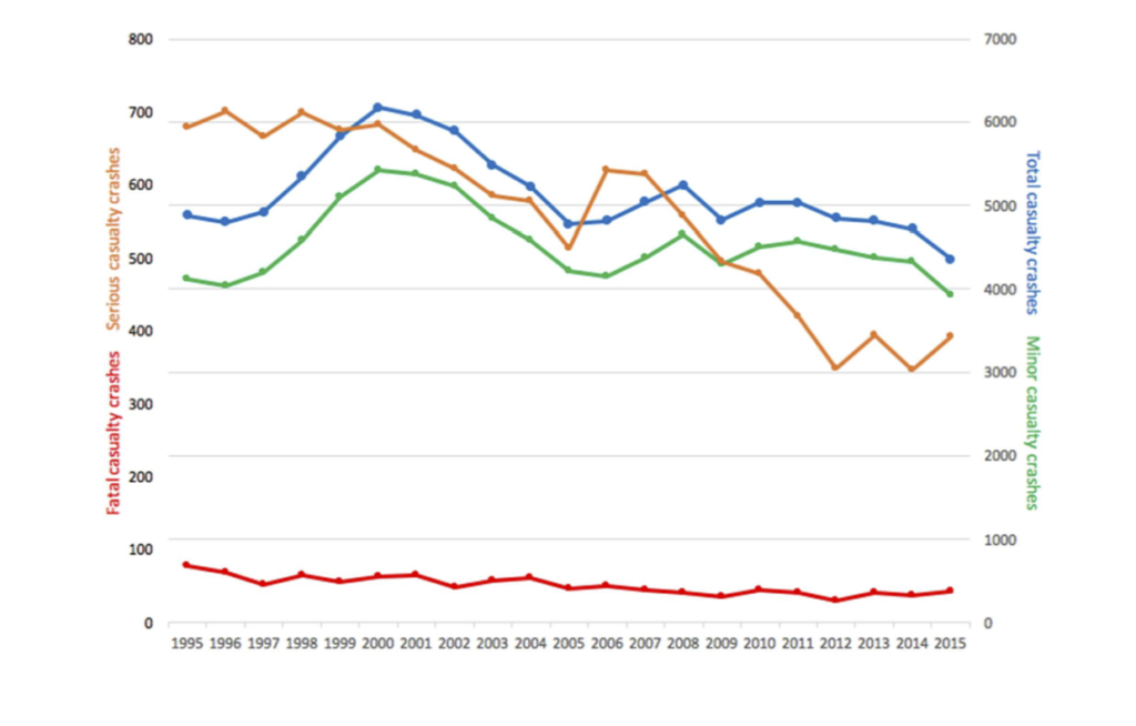
Figure 1: State-wide crash data by category.
The principal approach taken by the team was to compare the incidence of crashes before and after a camera was installed at an intersection. However, as just noted, there are likely to be other confounding factors that will also influence the before and after incidence of crashes. Some attempt needs to be made to try to account for these factors if we want to identify the effects of the safety cameras alone. Two possible methods were considered for defining a control or reference for this purpose. These will be described in more detail below.
RAA was able to provide the MISG team with the following data (mostly in electronic form).
- Complete detailed crash data from 1996. This is from police crash reports. Crashes are classified as property only or casualty, with casualty further divided into minor injury, serious injury (requiring para-medical treatment or hospitalisation) and fatalities.
- Offence (expiation) data collected from safety cameras since 2011. This is a record of speeding and red-light offences.
- The operational history of safety cameras, including location, start-of-service date and any subsequent out-of-service periods (for example, cameras usually need to be turned off if there are roadworks being undertaken nearby). This data is reasonably complete for cameras that are currently installed, though less complete for cameras that are no longer operational. (Older styles of cameras have been removed from some locations, and not necessarily replaced with newer style cameras.)
- Traffic flow information. Some estimates of traffic volumes on some major Adelaide metropolitan roads were available. These are usually only available as average data collected over a period of a week or so. This data was mostly in paper form.
The team decided to focus only on casualty crashes, that is, property damage only crashes were excluded from consideration. The reason for doing this was that crashes involving casualties are the most serious kinds of crashes.
It was realised, however, that by doing this the MISG was in effect concentrating on minor injury crashes, since, on a state-wide basis at least, Figure 1 shows that minor injury crashes are around 90% of casualty crashes. It was also noted that Figure 1 shows a noticeable difference between the year-by-year patterns for minor injury and serious injury crashes.
On the advice of the industry representative the team also decided to only consider the 90 current safety cameras that are installed at intersections. (The remaining 82 cameras are at pedestrian crossings or straight road sections.) Among these intersections are 25 of the 40 worst signalised intersections for casualty crashes since 1996.
After this initial review of the RAA problem, the MISG team formed into a number of sub-teams that each addressed a different aspect of this overall problem. The activities of these sub-teams will be described in the following section of this summary report
Sub-team Activities
Poisson model of road crashes
The occurrence of crashes at an intersection is often presented as a classic textbook example of a Poisson process. A Poisson process is a random process that is characterised by a fixed probability of an ‘event’ occurring during a unit of ‘time’, or unit of some time equivalent. In the case of traffic crashes, this would be a fixed probability of a crash for each vehicle passing through the intersection. (Traffic flow here is the time equivalent.) If a Poisson process model were to hold, then the number of crashes per 100,000 vehicles (say) would satisfy what is called the Poisson distribution. To become specific, let λ be the probability that a vehicle passing through the intersection will have a crash. The average number of crashes per 100,000 vehicles would be 100,000 λ. Since the occurrence of a crash is a random process, the actual number of crashes per 100,000 vehicles will vary about this mean. This magnitude of this variation can be quantified by the standard deviation of the Poisson distribution, which is a kind of ‘error bar’ indicating the expected variability. One property of a Poisson distribution is that its standard deviation is the square root of its mean. So, for example, if the mean number of crashes at an intersection per 100,000 vehicles was 10, then the standard deviation would be close to 3.2.
The casualty crash data for all intersections with cameras was investigated to see whether it was consistent with a Poisson model. However, it was found that the annual count data showed considerably greater variability from year to year than could be reasonably explained by a simple Poisson model, even accounting for a possible before and after camera installation change in the Poisson parameter. The possibility of a time-dependent Poisson parameter was considered, but it was not explored further. The sub-team concluded that there was considerably greater variability in the data than could be accounted for just on the basis of a simple Poisson process model.
In hindsight, this is perhaps not too surprising as the underlying Poisson assumption that each vehicle passing through an intersection has the same probability of a crash sounds rather simplistic. It would be expected, for instance, that some vehicles, or rather the drivers of those vehicles, would engage in riskier driving behaviour and so would be more likely to be involved in a crash than other vehicles and drivers. The proportion of risky vehicles would itself likely be probabilistic, and so there would be multiple interacting probabilities at play, rather than the simple case envisaged by a Poisson process. The resulting distribution would therefore likely be rather complex.
Road crash variability at the individual intersection level
Annual casualty crash data at the level of an individual intersection was also investigated by other sub-teams. These investigations showed that such individual intersection count data was very noisy. This was not surprising, since a casualty crash is a rare event that occurs randomly in time. This convinced the team that in order to make progress the data would need to be aggregated, that is, averaged over time or over intersections (or both).
From a statistical point of view the advantage of such aggregation of data is
- the distribution of aggregated quantities is typically closer to a normal distribution than is the underlying distribution
- the variability (standard deviation) is reduced by aggregation.
However, on the other hand, an aggregated analysis means that it is no longer possible to look at the properties of individual intersections.
The initial request from RAA asked the MISG to look at crash data at the level of individual intersections. Because of the above considerations, this original scope of the problem needed to be modified.
Before and after analysis—state-wide data as reference
For the intersections currently with safety cameras the average numbers of casualty crashes per year before and after the installation of the current camera were calculated. These results are presented graphically in Figure 2, where a red vertical bar is used to indicate the before-installation average and a blue bar shows the after-installation average. (Only data post 2001 was analysed as there was not reliable installation data prior to this.) For each intersection the blue bar was laid over the red bar; so if a bar is of mixed colour, with the red still visible above the top of the blue bar, it indicates that the before-installation average is greater than the after-installation average; if only blue shows, it indicates that the after-installation average is greater than the before-installation average. Note that for 17 of the intersections there was no red bar present, as these cameras had been in place for the entire period since 2002. It is seen that for the majority of cases, the red (before-installation) average is greater, which suggests that the installation of a camera leads to a reduction in the number of casualty crashes.
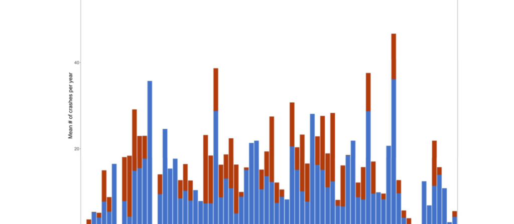
Figure 2: Comparison of before-installation and after-installation average annual casualty crashes for the intersections currently with safety cameras installed.
However, in this simple analysis the data was not adjusted to account for any underlying time effects, such as changes in state-wide traffic volumes (Vehicle Kilometres Travelled) or the general state-wide reduction of casualty crashes with time mentioned earlier.
This data was analysed again making these two adjustments, and produced a broadly similar result. However, care needs to be taken in interpreting this result since there is considerable variability in the number of casualty crashes from year to year anyway, even without any consideration of the introduction of a safety camera. It could possibly be the case that the observed fall in casualty crashes after the introduction of a camera is just an instance of this underlying variability, with the safety camera itself having no effect. To test whether this might be the case, a simple test of statistical significance, the sign test, was applied.
The mathematical background to this test is as follows: Suppose the introduction of a safety camera had no effect. This could be stated mathematically by saying that the probability that any intersection has a greater number of casualty crashes before the introduction of the safety camera than after the introduction of the safety camera is 50%, and likewise, the probability of there being a lesser number of casualty crashes before the introduction of the safety camera than after would also be 50%. The observed proportion of the 58 intersections that have a greater number of casualty crashes before compared to after is actually around 86%. The significance test gives the probability p that a proportion of 86% or more would be observed in a group of 58 intersections assuming that for each intersection the probability that a greater number of casualty crashes occur before the introduction of the safety camera than after the introduction of the safety camera is 50%.
If this probability is considered ‘small’, then it is concluded that it is highly unlikely that the probability is 50%, and that therefore it can be reasonably asserted that there has been a ‘real’ (statistically significant) change in the number of casualty crashes. (Note that there needs to be a slight refinement of this explanation to account for the case of exact equality of before and after casualty crash counts.)
In the present case, with the adjusted data, p ≈ 10-6; that is, there is only a one-in-a-million chance that the observed proportion would result from pure chance. So it can be reasonably concluded that the introduction of the cameras is associated with a statistically significant change in the number of casualty crashes.
Furthermore, a preliminary analysis suggested that there was on average a 25% reduction in casualty crashes after the introduction of a safety camera. However, further work needs to be done to confirm this. It needs to be kept in mind that the adjustment of the data has used state-wide factors. Such state-wide factors may not necessarily be appropriate for the particular intersections being considered.
Another analysis was carried out looking at the proportion of casualty crashes that are in the serious injury or fatality categories. Using the 90 intersection data, all the before-camera installation casualty data was combined, and all the after-camera installation casualty data was combined. Of the before-camera casualties, 9.6% of these casualty crashes were serious injury or fatalities. On the other hand, of the after-camera installation casualties, 6.7% were serious injury or fatalities. In this analysis, this difference was statistically significant. However, a different method of analysis, using a different data set, could not detect a significant difference in this proportion. This question therefore requires further analysis with more complete data.
This analysis presents another possible way of assessing the influence of safety cameras. It has a statistical advantage in that it should be relatively insensitive to underlying time effects and the other potential confounding factors mentioned earlier, as long as it is supposed that these will affect all categories of casualties in the same way. It also raises the interesting speculation that the presence of a safety camera may have different effects on different categories of casualties, and, by extension, crashes more broadly.
Before and after analysis—reference group of ‘similar’ intersections
An alternative ‘before and after’ approach was also investigated. This looked at 96 high traffic volume intersections on arterial roads in the Adelaide metropolitan area. These were all considered to be ‘similar’ in nature. (These intersections were chosen by the industry representative.) Casualty crash data is available from 1996 onwards for all these intersections. Of these intersections, 35 currently have safety cameras, which have been progressively introduced since 2001. Some of these intersections have more than one camera; however, this extra degree of detail was disregarded and each intersection was classified as either having one or more cameras, or having no camera. Thus there are 61 intersections that have never had cameras in service at any time during 1996 — 2015. This set of intersections provided the reference group of intersections. From the 35 intersections currently with one or more cameras, two groups were chosen.
- Group A: safety cameras first installed in 2001 or 2002 (11 intersections)
- Group B: safety cameras first installed in 2006 or 2007 (11 intersections).
For each of Group A and Group B we considered the five-year time period immediately before and the five-year time period immediately after the safety camera installation. (As most cameras were installed part way through either 2002 or 2007, these years have been excluded from the time periods.) For each group and each five-year period the annual number of casualty crashes per intersection was averaged over all intersections in the group and over the five-year period. Corresponding averages were also calculated for the reference group. Results are shown in the table below.
| Group A (n = 11) | Group B (n = 11) | ||||
|---|---|---|---|---|---|
| 1997–2001 | 2003–2007 | difference | 2002–2006 | 2008–2012 | difference |
| 8.62 | 7.38 | 1.24* | 6.22 | 5.53 | 0.69 |
| (0.59) | (0.65) | ||||
| Reference (n = 61) | Reference (n = 61) | ||||
| 1997–2001 | 2003–2007 | difference | 2002–2006 | 2008–2012 | difference |
| 4.45 | 3.58 | 0.87* | 3.72 | 3.70 | 0.03 |
| (0.25) | (0.22) |
Mean number of casualty crashes per year per intersection averaged over the indicated five-year periods for intersections in Group A and Group B. Corresponding averages for the reference group are also given. The column named ‘difference’ shows the difference: earlier period – later period; and the quantity in parentheses is the estimated standard deviation of this difference. (An asterisk * denotes a statistically significant difference, p < 0.05.)
For the reference group there is a decrease in the average number of casualty crashes per intersection between the 1997–2001 period and the 2003–2007 period. This difference is statistically significant, as it is more than three times the estimated standard deviation of the difference. Note however, that this is not the case for the difference between the 2002–2006 and 2008–2012 periods for these reference intersections. In this case, the difference, although a decrease, is not statistically different from zero. This is also the case for the Group B intersections, where, again, there is a decrease in average casualty crashes between these two 5-year periods; however, this difference is comparable to the estimated standard deviation of the difference, and so we cannot conclude, with any confidence, that this difference is statistically different from zero. For the Group A data, there is also a decrease from the 1997–2001 period to the 2003–2007 period. In this case we might have greater confidence that this difference is statistically different from zero as a one-sided t-test gives p < 0.05.
Notice that the mean number of casualty crashes for the Group A intersections is greater than the mean number of casualty crashes for the reference intersections for both the five-year period before and the five-year period after the installation of the safety cameras. This is perhaps not unexpected, since safety cameras are preferentially installed at high risk intersections. One possible way of measuring the possible effect of cameras is to compare the ratio of the mean number of casualty crashes at Group A intersections to the mean number of casualty crashes at the reference intersections for the five-year periods before and after the installation of the safety cameras. Using the data from Table 1 gives
| 1997–2001 | 2003–2007 | |
|---|---|---|
| mean (Group A) / mean (Reference) | 1.94 | 2.06 |
The statistics of these ratios is rather complex and was not able to be investigated during the MISG. Thus accurate confidence intervals were not calculated. However, because of the substantial variability present, it is unlikely that the two quite similar values above are statistically significantly different. So, on this basis, we are unable to say with any confidence that there has been any effect of the safety cameras by this ratio measure.
Year-by-year plots for Group A and Group B intersections and the reference group are shown in Figure 3. Note that the reference intersection data shows a broadly similar pattern as seen for the state-wide casualty crash data in Figure 1. It was noted that both the state-wide and the reference group casualty crash counts peak around the year 2000. For the state-wide count, this peak is largely caused by a peak in minor injury crashes at that time. This led to some discussion at MISG about the possible reason for this peak, with the speculation that there may have been a change in definition or policy related to the reporting of minor casualties around 2000. Another suggestion offered was that the change to a 50 km/h speed limit on some metropolitan roads may have been a factor, particularly influencing the reference intersections. Due to lack of time, this suggestion was not further pursued or checked to see whether it actually applied to the reference intersections around 2000.
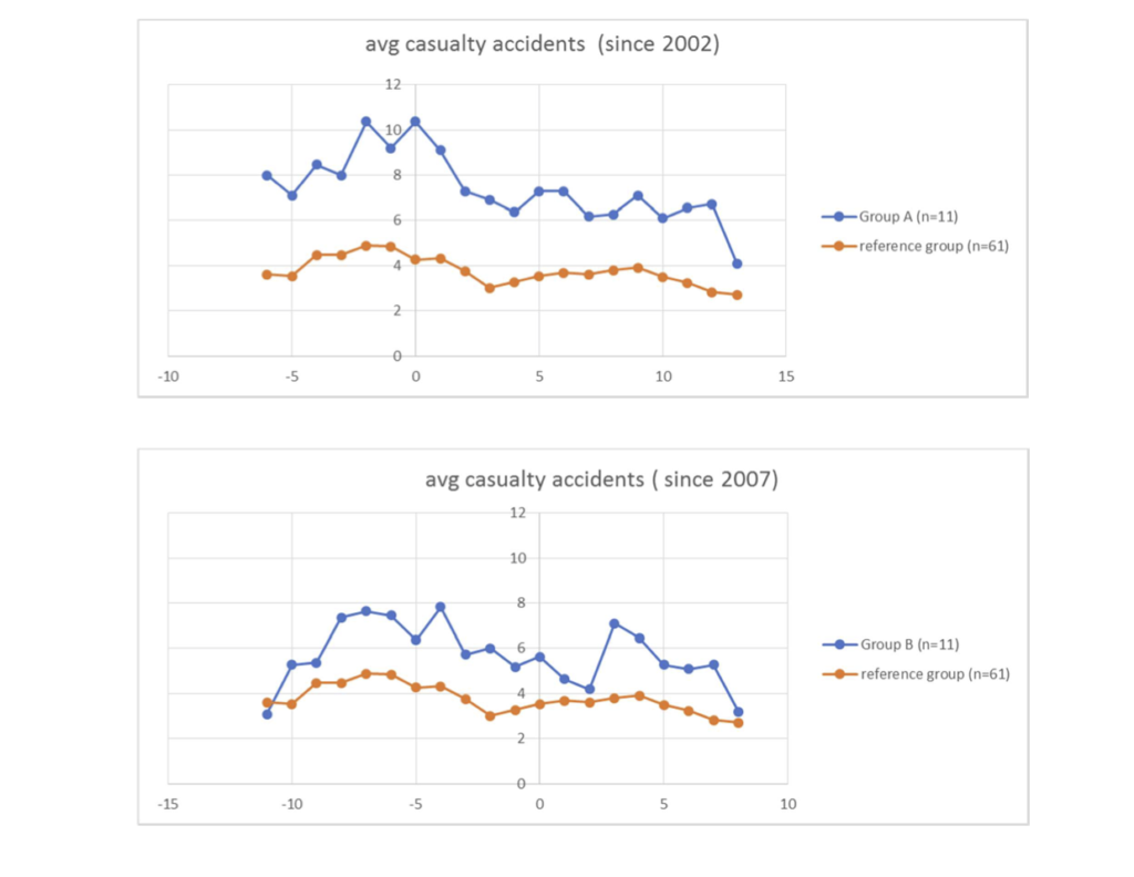
Figure 3: Year-by-year plots of average number of casualty crashes in Group A, Group B and the reference group
The statistically conservative interpretation of this analysis is that there was a decrease in the number of casualty crashes after 2001–2002 at both the reference intersections and the 11 intersections with the newly installed cameras. Whether the introduction of cameras was the cause of one or both of these decreases cannot be said. However, there seems to be something special about this 2001–2002 change event. For 2006–2007, when a second batch of 11 cameras were introduced, there was no statistically significant change in the number of casualty crashes between the before and after periods for both the Group B and the reference group of intersections. We could perhaps speculate that the introduction of the first batch of safety cameras had both an effect at the Group A intersections, which had the cameras, and more widely in the metropolitan area, as represented by the reference intersections. The introduction of the second large batch of cameras, on the other hand, had no noticeable effect. To further refine this analysis, and hopefully obtain more definite conclusions, it would be necessary to analyse the complete data sets that RAA provided. The team was only able to consider a subset of this data during MISG week.
Simple analysis of some expiation data
Extensive offence data that was collected by the 90 safety cameras was available. This data recorded offences, namely speeding or red-light offences. One sub-team looked at the question of whether offences were correlated in any way with casualty crashes. The motivating idea was that intersections with high casualty crash counts may also be associated with riskier driver behaviour, and that this would be indicated by a higher rate of offences. Results are shown in Figure 3 broken down by offence type. There appears to be little correlation of offences with number of casualty crashes. Had there been a correlation, the data in these plots would cluster around a line, indicating that intersections with high casualty crash counts would also tend to have high offence counts.
This lack of correlation seems a little surprising. One possible explanation could be that the behaviours that safety cameras target are not necessarily the behaviours that primarily cause crashes at these intersections. Note that there are also many more recorded offences than casualty crashes. So, there must be some other ‘missing’ factor(s) which needs to be present in addition to one or both of the targeted behaviours in order for a casualty crash to occur. This factor might be driver inattention or misjudgment, possibly exacerbated by alcohol. One might speculate that most offences could be called ‘calculated’ offences—that is, the driver has made a calculated assessment that they can ‘safely’ offend without causing a crash.
For example, a driver may conclude that they can turn right on a red arrow safely before any opposing traffic stream commences, or that speeding up to beat a red light is safe to do in some specific traffic situation. It is only when this calculation is wrong, that a crash is likely.
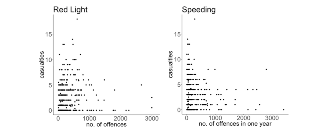
Figure 4: Correlation between offences (red light offence and speeding) and casualty crashes. Each data point represents one year of data for an intersection.
Traffic flow analysis
Detailed traffic flow data, some of it hourly, was available for a small number of Adelaide CBD intersections. One sub-team looked at this data to see whether there might be a correlation between traffic volumes and casualty crashes. The conclusion was that for each intersection they investigated, most crashes occurred at medium traffic density. An intuitive explanation for this is that at high traffic density, average vehicle speed is low, and so crashes are less likely. On the other hand, at low traffic density, crashes are also less likely to occur since there are fewer vehicles on the road to be involved in crash. At intermediate traffic densities, there is a critical mix of number of vehicles and vehicle speed that tends to maximise casualty crashes.
Summary
The main conclusions reached by the MISG team during the week were:
- The variability in casualty crashes is considerably greater than can be predicted by classical Poisson process models.
- A variety of data analysis approaches suggest that the presence of safety cameras at intersections may be associated with a reduction in casualty crashes. However, further analysis is needed to firm up this preliminary conclusion. Due to the limited time available during MISG week, the available data was not able to be fully considered. In addition, some data relating to operational dates of some cameras was not available. RAA is trying to source this data from SAPOL.
During the course of the week some interesting speculation was also raised around:
- whether the presence of a safety camera may have different effects on different categories of casualties, or categories of crashes more generally; and
- whether the effect of a camera could really be localised to a particular intersection, or whether there was a wider zone of influence around an intersection within which the psychological effect of the safety camera was still present.
Contributors
The team that contributed to the RAA project consisted of: Richard Butler (RAA Representative), Bill Whiten, Claire Miller, Michael Lydeamore, Geetika Verma, Elizabeth Bradford, Jorge Aarao, Minjung Gim, Charles Lawoko, Peter Pudney, Colin Pease, John Ockendon, Amie Albrecht (Moderator) and Tony Miller (Moderator).