Planning electricity transmission networks

Industry representative: Bradley Harrison, ElectraNet

Moderators: John Boland, University of South Australia; Giang Nguyen, The University of Adelaide

Introduction

ElectraNet is an electricity transmission company, who operates 5,591 km of high-voltage electricity transmission lines in South Australia. In order to demonstrate value of infrastructure investments, the company is interested in performing a 20-year simulation of the development of the National Electricty Market (NEM) under various scenarios. These situations represent different possible eventualities in which gas price, the amount of carbon emissions reduction, and demand, will evolve over the next twenty years.

ElectraNet’s question is: how can we include the stochastic nature of renewables in the capital decision making process? Fundamentally, this ques- tion consists of two aspects: the inclusion of stochasticity into the network model, and the accuracy of such stochasticity. Our team was partitioned into two, each addressing one of the aformentioned aspects.

Stochasticity: inclusion

The current methodology of ElectraNet consists of two stages, both of which employ deterministic linear programming (LP). For each investment option and each scenario:

• In the first step, the company considers a reduced network model and apply a load-block approach, which averages the demand over relatively long time intervals. The problem is then modelled by a deterministic LP, the output of which is a generator expansion plan for the whole network. In this step, the cost of building interconnectors or generators can be calculated, in order to determine the capital savings.
• In the second step, the company performs a short-term simulation, using the generator expansion plan produced in the first stage. The full transmission network representation is employed, and simulated demand over shorter time intervals is used. This detailed model allows for the inclusion of losses and thermal limitations. The objective of this second step is to calculate fuel cost savings.

Collectively, the first and second steps estimate the savings from a particular investment option, under a given scenario. Observations from these simulations indicate that the load-block approach devalues interconnector developments, which can smooth out intermittency across the market. Thus, the current approach can be improved to take into account three factors: the randomness of generation outputs from wind and solar farms, the expansion of batteries and pumped storage, and the gradual retirement of conventional generators.

Randomness of generation outputs

For simplicity and clarity in exposition, we focus on the first step in ElectraNet’s current approach; however, the following approach also applies for the second step.

In order to incorporate stochasticity into the modelling, it is important to keep the randomly-varying generation outputs as close to their uncertain characteristics as possible, instead of following the load-block approach. This implies that the constraints in the linear program are stochastic, and thus the resulting model is a stochastic Linear Program. To solve this stochastic linear program, we suggest a mathematical framework called stochastic programming with recourse. The key idea is to solve the stochastic linear program in two stages:

• In the first stage, we consider only deterministic constraints, and solve the reduced deterministic linear program to find a so-called first-stage solution.
• In the second stage, we solve another deterministic linear program to determine the minimum expected recourse, that is, the minimum expected cost for satisfying the violations to the stochastic constraints if there is any.

The overall objective is to minimise both the deterministic costs, resulting from, say, capital and operational costs, and the expected recourse.

We demonstrated the methodology using two toy examples, one with two states (SA and VIC), and the other with five states (adding also NSW, TAS and QLD). The five-state example was to illustrate the scalability of the two-state version.

The two-state example showed that:

• Under the load-block approach, currently employed by ElectraNets simulations, the optimal solution was to build an additional generator at each location.
• In the stochastic programming framework, however, the optimal solution was to build an interconnector between the two states.

In this example, while the capital cost of building the interconnector is higher than building two generators (which explains why the deterministic LP favoured the latter), over time and on average the cost of meeting demand violations due to the stochastic nature of generation outputs is higher if one builds two generators instead of one interconnector. The longer the time horizon we consider, the larger this cost difference, assuming that the cost of operating generators is significantly higher than that of maintaining interconnectors.

Complexity of stochastic programming

The deterministic LP in the first step of ElectraNet’s simulations currently takes about three hours to solve. If we maintain the randomness of generation outputs in the model, the deterministic constraints involving these outputs will become stochastic constraints. In order to find the minimal expected penalty cost, we effectively have to solve a deterministic LP for each realisation of the random variables representing generation outputs; these LPs can be combined into one master LP to be solved simultaneously.

The two main factors to consider when solving these LPs are the number of realisations required to realistically approximate these random variables, and how to effectively handle the master LP. To address the first issue, we can employ Monte Carlo techniques based on sample average approximation. About the second, as the combined LP has a special block structure we can use a well-known linear programming technique called Benders decomposition, to divide and conquer the model.

Battery and pumped storage

We also introduced the option of battery and pumped storage into the toy model, taking into account the discharge ratio of battery storage. The optimal solution showed that having battery storage reduced the need for building new generators.

Understanding the input data

The Australian Energy Market Operator (AEMO) has provided what is termed as a representative data set comprising demand data plus several types of renewable energy supply. These demand and supply sets are for separate regions across the National Electricity Market (NEM). The supply variables include:

• wind farm output,
• fixed flat plate photovoltaic (PV) cells,
• single axis tracking PV cells, and
• dual axis tracking PV cells.

We have investigated the renewable supply data under the principle of whether it contains sufficient variability to adequately assess the various options in the long term planning process. Note that our understanding was that the 30 years of data is based on actual data from 2013-2014.

Wind farm output

We selected a single data set of each type of variable upon which to perform the assessment. For wind farm output, Starfish Hill Wind Farm in South Australia, southwest of Adelaide, was selected. The data is half-hourly power in Megawatts (MW), which we first converted into hourly energy (MWh). We assumed that power is constant over the half hour so the equivalent energy is in Megawatt half hours.
As we performed the analysis we noticed that the maximum daily output occurred on June 28 every year. Thus, we decided to compare the daily totals over all 30 years. To make the comparison easier we deleted leap days and also took the last six months of 2016 (the first part of the set) and positioned them at the last six months of 2046. When the yearly daily total values were plotted all on one graph, the result showed an interesting feature—the total energy for a given day is the same every year. In other words, we are only performing any optimisation on a single representative year of wind farm output.

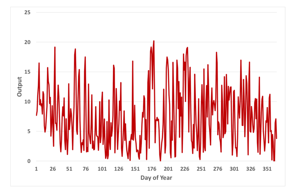
It would be better to take the wind farm output and use statistical and time series techniques to generate any number of years of synthetic data files that have the same gross statistical characteristics but may well contain some more extreme sequences than the original and thus allow us to test the performance of configurations under more demanding conditions.

Solar radiation

The original half-hourly solar radiation was converted to hourly and daily data for the years 2016–2045 for the City of Adelaide. To simplify the analysis of solar radiation data, leap days were removed. The analysis revealed a repetition with time shift as shown in the figure below.

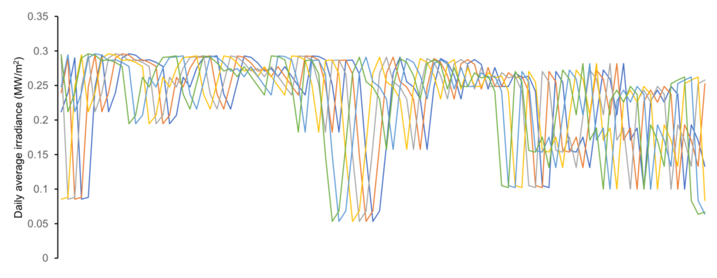
This result indicates that solar data for 2016–2045 is essentially one year of data repeated at random with a time shift up to 6 days. The time shift is probably induced to add stochasticity into the data that would allow analysing the sensitivity and the long-term performance of the system. However, the time shift is unlikely to generate reliable stochasticity as both deterministic and stochastic components of solar radiation are modified. Consequently, sensitivity and long-term performance of the system based on the time-shifted data are unlikely to be reliable. A similar recommendation is made for the wind data, in order to induce stochasticity.

Acknowledgements

The moderators and industry representative would like to thank the researchers who contributed to this work: Erika Belchamber, Elizabeth Bradford, Mark Carey, Lui Cirocco, Sleiman Farah, Joon Heo, Angus Lewis, Charles Ling, John Pockett, Rachael Quill, and Kirrilie Rowe.